Category Archives: Global

Good refractory practices are necessary to achieve proper refractory installation. It all begins with mixing. As discussed in the article “The Lost Art of Mixing Refractory,” published in the February 2008 issue of Insulation Outlook, it is common to find workers without previous experience mixing refractory at power plants.

If the workers installing the refractory have limited experience, they might not be able to react or adjust to a refractory mix that is not the correct consistency for the application. At a power plant, for example, the refractory mix brought to the point of installation was too wet (i.e., it had too much water) for the trowel application required. The lack of experience of those doing the installation meant that they did not know to wait a few minutes to allow the refractory to set up (or stiffen) before application. They were unaware that refractory has a pot life (the time recommended by the manufacturer between mixing and installation). The workers could have waited a suitable period (5 to 10 minutes) to get a better install with less mix falling off the vertical wall surface.

The refractory mix described above was mixed improperly. The extra water in the mix means that the refractory will have less strength and be more prone to failure even though it could be troweled onto the vertical wall surface (with difficulty).

Mixing refractory is not only about adding water to the mix using a hose and mixing it just enough until it looks wet—like mixing concrete. Mixing refractory requires a bit more. Properly mixed refractory must:

  1. Have a carefully calculated, measured, and/or weighed amount of water
  2. Never have water added directly from a water hose
  3. Be mixed for a certain amount of time
  4. Be mixed in a paddle mixer or by hand, vigorously
  5. Be mixed to the consistency matching the application of usage

To mix refractory properly, one must know the type of application intended for its use. The most common applications are casting, pouring, and troweling of refractory.

  • Casting and pouring applications are used for installing large amounts of refractory and usually require forms to hold the refractory in place. The mix consistency should include just enough water so the material will flow into the formed area. Using the ball-in-hand test, the mix should flatten out on the palm when tossed into the air.
  • Troweling application is used for hand-applied areas requiring thin linings. The mix consistency should have just enough water added so the material is sticky and will stay in place without falling off a vertical surface. Again, using the ball-in-hand test, the mix should flatten out on the palm when tossed into the air.

The following suggestions are listed to help those with less experience get a better refractory mix:

  1. Never use a cement mixer. Refractory mixed in a cement mixer will not have the strength characteristics expected by design. A cement mixer should only be used for adding the initial amounts of water to the dry mix. After all the water is added, the wetted mix must be emptied into a pan or tub and vigorously hand mixed for the total time required. Refractory needs the action created by the paddle or by the rigorous stroke of hand mixing to get the proper reaction required between the water and cement.
  2. Check the size (capacity) of the paddle mixer to be used and figure one bag fewer than the size or quantity of bags the mixer is designed to mix. Paddle mixers are usually based on capacity (two, four, or six bags are common sizes). The paddle mixers are very temperamental and can jam easily, especially if they are not used every day. Using one fewer bag will eliminate the tendency to jam.
  3. Calculate the amount of water recommended by the refractory manufacturer. This is normally printed on the back of the refractory bag and will be either a percentage of weight or a measurement (quarts, pints, gallons). The recommended amount of water on the bag is usually for casting, which should be noted if the application is to be troweled. Figure 1 gives an example of such a calculation. This type of chart or conversion calculation can be used for developing or establishing the
  4. Pour expected water amounts into clean buckets or pails, following the procedures in “The Lost Art of Mixing Refractory” (Insulation Outlook, February 2008). The first mix/batch will establish the exact amount of water needed, so keep a measured or weighed gallon of water off to the side in case more water is needed to reach the consistency the application requires. Remember, you can never be too accurate in establishing the initial water quantity. (There is no shame in using a bathroom scale to measure initial water amounts.)
  5. Test for proper mix consistency using the ball-in-hand method and note the exact amount of water used (or not used); then, refill the buckets or pails with the total amount of water used to complete the first batch/mix.
  6. Place a mark on the outside or drill small holes in the pails or buckets. These pails or buckets then can be used to ensure mix/batch consistency. If properly marked or labeled (with refractory material name and application), and stored so they remain clean, they can be reused for similar work.
  7. Add the water, following the procedures in “The Lost Art of Mixing Refractory” (Insulation Outlook, February 2008). Keep in mind that a properly mixed refractory material most often will appear to be on the thick side. That is the desired consistency.
  8. Mix the refractory based on good refractory procedures, such as those in “The Lost Art of Mixing Refractory.” Avoid adding too much water, even though that may make the mix easier to handle. Too much water robs the refractory material of its strength.
  9. Use a watch or timer when mixing refractory, because over-mixing or under-mixing also robs the refractory material of its strength.

Mixing refractory properly means using the exact amount of water–not guessing or approximating. Proper mixing means mixing for the correct amount of time, providing the refractory to the point of installation in the right consistency, and having the mix retain its consistency until the installation is complete. Anything less is an improper mix and is usually the root or contributing cause of refractory failure.

Paying attention to the mixing process and keeping the consistency of each batch will help ensure that a proper refractory installation is off to a good start. Though refractory may be among the smallest components on a steam-generating boiler, it is one of the most important for keeping the fire inside the box and for energy efficiency. To achieve better refractory installations, review refractory mixing practices to avoid refractory failures and application problems.

Figure 1

The power industry’s operating and maintenance practices were held to intense regulator and public scrutiny after November 6, 2007, when a Massachusetts power plant’s steam-generating boiler exploded and three men died.

The Commonwealth of Massachusetts Department of Public Safety’s Incident Report investigation determined that the primary cause of the Dominion Energy New England-Salem Harbor Station Boiler #3 failure was extensive corrosion of boiler tubes in the division wall at the east furnace lower slope dead air space (Figure 1). The three operators were working directly below the furnace on a pulverizer seal air fan when the explosion occurred. They died of burns and related complications. The boiler was operating at 1,900 psi at the time of the failure. A complete set of photos of the failure is included in the Incident Report.

The report concluded that when the tubes failed within the dead air space formed by the division wall—an area normally under a slight negative pressure—the vestibule was instantly pressurized, causing a secondary rupture of the boiler casing around the bottom of the furnace. Ash and 600°F steam then were released into the area where the three workers were (see Figure 2).

The report summarized interviews with plant staff on standard plant operating and maintenance habits. Because the plant has operated as a cycling unit for about 10 years, planned outages were so reduced in length that required maintenance activities were not completed. At the time of the accident, approximately 2,500 work orders were pending.

The report also noted that the dead air space had not been opened or inspected in at least 10 years and was full of ash at the time of the explosion. The report concluded that the tube explosion that blew out the outer wall of the furnace was caused by ash and water from boiler washing coming into contact with tubes. That mixture caused corrosion that resulted in excessive tube metal loss.

The report held the chief engineer and the outside boiler inspector directly responsible for the explosion because they failed to perform a comprehensive inspection as required by Massachusetts law. The catastrophe could have been prevented if proper inspections had been made of the entire furnace and if more than visual inspection techniques had been used. The Occupational Safety and Health Administration has since found 10 serious safety violations at the plant, including failure to enter and inspect the area where the tube rupture occurred.

It would be a mistake to close the book on this tragedy now, chalking it up to bad luck on the part of the plant’s staff. There is much more to the story than what is written in the Incident Report. The key question the report failed to answer is: What caused the vestibule to fill up with fly ash in the first place?

The argument could be made that the root cause of the accident was refractory failure that allowed the water and ash to enter the vestibule in the first place. A properly installed and maintained refractory surface would have prevented the corrosion and, thus, the accident.

Good Boiler Design Practice

The report states that the boiler’s lower vestibule was full of ash, and had been for a very long time. Post-accident operator interviews suggest the ash may have been there as long as 10 years. Poor maintenance and inspection practices left this enclosed space ignored. Unfortunately, this lack of attention is common throughout the power industry.

The boiler itself is a 1957 vintage 120-MW coal-fired radiant power boiler. This was a common design for virtually all utility boilers built from the mid-1940s through the 1960s. (It was not until 1964 that the membrane tube wall design was developed and became the norm in utility boiler practice.) Approximately 400 boilers of this design were built in the United States, and most are still in operation. All these boilers had similar steam capacity, tube wall construction, vestibules, and refractory/tube wall design (see Figure 3).

These are considered flat-studded or tangential-type boilers. They do not have membrane tube walls, but instead use either flat-studded tubes or bare loose tubes to form the boiler and furnace walls. To keep the fire (and fly ash) inside the firebox, refractory is applied over the outside of the tubes to form a protective, insulating wall.

Boilers of this type used either an “all-refractory design,” with refractory (1 to 2 inches thick) on the back side of the tubes, or an “inner-cased design,” which uses a thin layer of refractory applied flush with the back side of the tubes and a 10-gauge metal casing installed over the refractory-backed tubes. The all-refractory design was less costly, especially in areas such as vestibules and enclosures, and was therefore more commonly used. This discussion focuses on the all-refractory design.

In essence, the refractory must keep the fire inside the box to keep the boiler operating efficiently and to prevent fly ash from penetrating or entering the vestibules in and around the boiler.
These vestibules and enclosures are typically located under the superheater area, above the roof tubes, under drums, around the burner area, and below or just underneath the furnace hopper slope tubes (where the failure at Salem Harbor Station Boiler #3 occurred).

Designers and manufacturers of these types of boilers knew that it was very important to keep fly ash out of these vestibules because of its chemical constituents. Fly ash is a by-product of burning coal and typically contains alkalis such as sodium and potassium, which can form corrosive mixtures in the presence of water, or sulfur, which can form sulfurous or sulfuric type acids—both of which can corrode or weaken structural supports and tubes in the presence of water. The photos illustrate these points in a boiler similar to Salem Harbor Station Unit 3’s in design and construction.

Poor Refractory Practices

Boilers of this vintage and design use refractory on the back side of tubes inside vestibules and enclosures. The refractory is approximately 1 inch thick from the face of the tube and requires a support system. It can fail for any number of reasons, including:

  • Poor refractory mixing and handling practices
  • Poor installation practices (including curing and drying)
  • Improper water-washing techniques
  • Improper refractory attachment systems

The way to prevent failure is to mix, handle, and install refractory correctly, and follow proper water-washing practices. Refractory mixing, handling, and installation errors can be eliminated by following the guidelines provided by any reputable refractory manufacturer and following common industry practices for installing the refractory. Refractory destruction by water washing can be avoided by not water washing in areas where vestibules and enclosures are directly behind the waterwall tubes. If water wash must be done, then it should not be sprayed directly into the refractory, which is located between the tubes.

Unfortunately, many plants have an improper refractory attachment system, which is by far the most common reason for a refractory failure inside vestibules and enclosures. A refractory attachment system will support the refractory, even during boiler expansion, regardless of whether the refractory is installed using the gunning method (uses pressure to force dry material from the charging chamber through a hose to the point of placement; water is added at the discharge nozzle) or the trowel method (requires application of refractory by hand).

Most plants pay little or no attention to the attachment system for holding refractory inside vestibule areas. The most common practices for holding expanded metal at power plants are as follows.

  • No support system. The refractory will not last very long without a support system because of the stresses associated with boiler expansion.
  • A light-gauge attachment with clips. This application uses a thin-gauge attachment with insulation-type speed clips to support the expanded metal. This design is better for supporting ceramic module insulation applications than for refractory. The thin gauge of the stud and clip does not last long when exposed to stresses associated with boiler expansion.
  • Welding directly to the tubes. This approach does not provide sufficient support of the refractory because most of the refractory material is above the expanded metal. Given the stresses associated with boiler expansion, expanded metal should be placed in the middle of the refractory to give the optimum support.
  • The stud and clip method. This is a good method for holding expanded metal, as long as a clip is placed both under and above the expanded metal. The clip should be a heavy-duty speed clip (such as SN3) large enough to cover the diamond shape of the expanded metal openings. The problem with this system is the difficulty of keeping the expanded metal the same distance from the tube face. The distance of the expanded metal from the tube face is critical for the success and longevity of the system.
  • A hex nut and threaded stud with washers. This system is a variation of the stud and clip but uses hex nuts and washers for holding the expanded metal instead of a speed clip. This is a good method as long as the washers are placed both under and above the expanded metal. As with the stud and clip method, the heavy-duty (12-gauge minimum) washers should be large enough to cover the diamond shape of the expanded metal openings. The problem with this system is the difficulty of keeping the expanded metal the same distance from the tube face. The distance of the expanded metal from the tube face is critical for the success and longevity of this system.

A properly supported refractory should last 10 years or more if the refractory is installed (and dried) correctly. All the systems mentioned above have some drawbacks that could compromise the strength of the refractory support system and, consequently, affect refractory longevity.

Better Practices

Here is a method for holding 1-inch-thick refractory over the back side of tubes inside a vestibule or enclosure that has the best chance for lasting 10 years or more:

  1. Weld a 1/2-inch carbon steel hex nut face down (not on its edge) directly to the tube face on 12-inch horizontal x 18-inch vertical for flat areas and 12-inch x 12-inch centers on sloped or overhead areas. The 1/2-inch nut will act as a standoff, so the expanded metal will be located exactly in the middle of the refractory.
  2. Weld 1 1/2-inch x 9-gauge (13-gauge minimum) non-flattened expanded metal directly to the hex nut. Using this size of expanded metal will allow both the fine and course aggregate grain to penetrate through the expanded metal. Using a smaller size of expanded metal will cause a separation between the fine and course grains in the refractory, which reduces the strength of the refractory and will affect its longevity.
  3. The expanded metal should be overlapped by 1 inch to 3 inches in all directions. This overlapping helps locate the expanded metal so welding is possible at all hex nut locations and will take up the stresses associated with boiler expansion. The expanded metal is never welded in the overlap areas.
  4. Apply a medium-weight 2,000°F minimum, 45-percent alumina cement-bonded refractory 1 inch over the face of tubes through the expanded metal. It takes approximately an additional 1/2-inch thickness of refractory to completely cover the expanded metal. Remember that using more refractory than required does not give you a stronger or better refractory application.
  5. Cure the installed refractory for 24 hours by spraying/wetting the surface of the refractory with water every 2 hours, or by spraying/painting the surface of the refractory with water-based acrylic curing and sealing compound.
  6. Dry the refractory during boiler start-up by raising the boiler temperature 75°F per hour until the water/steam temperature inside the furnace wall tubes reaches between 250°F and 400°F, and hold it there for 2 hours. This will drive out the mechanical water used in the mixing process from the refractory. Then, take the boiler up at 75°F per hour to operating temperature.

Look to the Future

The root cause of the tragedy in Massachusetts could have been identified as refractory failure rather than tube failure. It was the failed refractory lining that allowed fly ash and water to penetrate into the lower furnace vestibule. The natural consequence of large ash deposits mixed with water and packed around boiler tubes was preventable.

The tragedy also never would have occurred if proper boiler inspection and maintenance practices had been followed. Everyone working in or affiliated with the power industry must do his/her part to make sure this kind of accident will never happen again.

The industry can honor the memory of those lost and ensure that a similar accident never occurs again by:

  • Ensuring that boiler outages allow sufficient time for inspection and repair of refractory
  • Following proper procedures for handling and installing refractory
  • Paying close attention to the refractory support system inside vestibules
  • Allowing enough time during boiler start-up procedures to dry the refractory
  • Avoiding water-washing tube walls in vestibule areas
  • Regularly inspecting vestibules and dead air spaces and quickly repairing damaged refractory
Figure 1

A tube rupture on November 6, 2007, at Dominion Energy New England’s Salem Harbor Generating Station Unit 3 caused a furnace explosion that killed three men. Source: Commonwealth of Massachusetts Department of Public Safety Incident Report: Dominion Energy New England–Salem Harbor Station Boiler #3 Failure, dated July 31, 2008

Figure 2

The Commonwealth of Massachusetts Department of Public Safety’s Incident Report found that extensive corrosion of the boiler tubes, caused by ash captured in the lower slope air space that mixed with water introduced by furnace washes, was the cause of the explosion. Source: Commonwealth of Massachusetts, Department of Public Safety Incident Report: Dominion Energy New England–Salem Harbor Station Boiler #3 Failure, dated July 31, 2008

Figure 3

A typical 1957-vintage one-pass boiler susceptible to a failure similar to that experienced at Salem Harbor Station Boiler #3. Approximately 400 of these boilers are in active service today. Source: BRIL Inc.

Figure 4

Ash inside the vestibule of the boiler at Dominion Energy New England–Salem Harbor Generating Station Unit 3.

Figure 5

Ash inside the vestibule of the boiler at Dominion Energy New England–Salem Harbor Generating Station Unit 3.

Figure 6

Refractory must keep the fire inside the box in order to keep the boiler operating efficiently and to prevent flyash from penetrating or entering the vestibules in and around the boiler. (These photographs were not taken at Salem Harbor Unit 3 but at units of the same boiler design and configuration.)

Figure 7

Refractory must keep the fire inside the box in order to keep the boiler operating efficiently and to prevent flyash from penetrating or entering the vestibules in and around the boiler. (These photographs were not taken at Salem Harbor Unit 3 but at units of the same boiler design and configuration.)

Figure 8

Vestibules and enclosures are typically under the superheater area, above the roof tubes, under drums, around the burner area, and below or just underneath the furnace hopper slope tubes.

Figure 9

No support system

Figure 10

Light-gauge attachment with clip

Figure 11

Welding directly to the tubes

Figure 12

The stud and clip method

Figure 13

The hex nut and threaded stud with washers

Figure 14

Overlapping aids welding at hex nut locations.

The building industry is experiencing an accelerating pace of change around energy efficiency. Utility and fuel price volatility, coupled with efficiency initiatives from many sources, are driving changes at a rate that may make many building projects, currently under design, out of date before they are built. Architects must consider this trend as they choose whether to meet today’s standards or prepare for tomorrow by meeting insulation standards that are certain to exist in the near future.

The most immediate change is the release of the new edition of ASHRAE 90.1.1 The 2007 edition was published in January of 2008 containing significant increases in energy efficiency requirements. Originally scheduled for release in June of 2007, the U.S. Department of Energy (DOE) urged ASHRAE to delay publication so two addenda (one for opaque envelope components and another for fenestration) could be included to accelerate their contribution to national energy savings.

The 2007 standard will likely be referenced in the 2009 International Energy Conservation Code (IECC) and then be considered for adoption by local code jurisdictions. Since many communities only adopt code updates in harmony with the three-year International Code Council (ICC) publication cycle, it was important to get the updated energy efficiency standard in place in time to make the 2009 edition of the IECC. All of this is happening in advance of the publication of ASHRAE 90.1?2010, which has the goal of achieving a 30-percent energy savings compared to the base ASHRAE 90.1?2004 edition. With energy codes changing rapidly, and with other sustainability initiatives gaining momentum daily, it makes sense to insulate at levels higher than code minimums so your project is not “energy-out-of-date” before the client moves in.

Sustainability and Energy Efficiency

In 2006 the American Institute of Architects issued its 2030 Challenge. It called for an aggressive and relentless improvement in energy efficiency until buildings become carbon neutral and do not use fossil fuel or greenhouse gas-emitting energy to operate by the year 2030. The Challenge was soon endorsed by the U.S. Conference of Mayors, and a host of agencies have pledged to help set the benchmark to measure improvement. This goal is very aggressive and will require significant innovations in the way buildings are built and operated. Buildings under design today are likely to still be in use in 2030. Therefore, it makes sense to consider future energy efficiency goals as you specify insulation today.

On another front, most green building initiatives place a high value on the role of energy efficiency. For example, Leadership in Energy and Environmental Design (LEED) 2.0 is a green building rating program developed by the U.S. Green Building Council. It places a very high priority/reward on exceeding ASHRAE 90.1 minimum standards. During the design phase for projects, many design professionals consider the objectives of LEED, even if they do not plan to pursue LEED certification. So if a user couples rapidly advancing energy efficiency standards with the increasing prominence of LEED sustainability goals, it is not difficult to imagine that a current project may be “energy-out-of-date” before the client moves in.

It’s possible to prevent out-of-date projects and best serve building owners and occupants by anticipating changes that surely will only grow over time due to energy volatility and the associated increased energy costs. So position your client’s building for the market demands of the very near future by designing it to operate competitively with low energy costs.

From “Common Practice” to
“Investment Analysis”

Keep in mind that increased insulation requirements in codes and standards are not arbitrary or “nice to do”; they are justified by economic considerations. Higher levels of insulation are warranted by the cost of energy saved, which also translates into a lighter environmental footprint of the building. Let’s examine a brief history of energy code economics.

When the original “Standard 90” was developed in the mid-1970s, requirements were based on established or “common” construction practices. Within 10 years, all 50 states enacted regulations based on Standard 90. Throughout the 1980s, research continued in the areas of energy efficiency, fuel calculation techniques, and dynamics between various building components. All of those developments led to issuance of the first ASHRAE Standard 90.1 in 1989.

Drawing upon lessons learned and criticisms from the development of the initial standard, ASHRAE began early in 1990 to evaluate criteria for the next version of the standard. Two key decisions were made:

  • Economics should be used as the basis for setting the criteria
  • All sections of the new standard should apply the economic approach to ensure the standard is balanced among building components, such as envelope, lighting, and mechanical

The 1999 edition, as well as the subsequent 2004 and 2007 editions, was based on these two economic concepts.

In recent editions, ASHRAE 90.1 has used an “investment analysis” or an “investment approach” to calculate “optimum” insulation levels and establish those as the minimum levels. “Optimum” or “lowest life-cycle cost” insulation levels are calculated based on assumptions made about present and future market conditions (first cost of installed insulation, life-cycle cost of energy, present and future cost of money, etc.). One method to predict future trends is to plot past costs and project similar trends into the future. That method depends on fitting curves to historical data, which may lead to less accurate predictions because parts of the curve vary greatly in rate of change over the years as cost trends vary. Another method, the one adopted by ASHRAE, uses economic scalar ratios, which combine many complex variables and their historic fluctuations into a factor that simplifies the calculation and avoids the difficulty in selecting specific economic parameters for building components.

Scalar ratios expand the traditional
life-cycle cost concept of uniform present worth factors to account for non-uniform fuel escalation rates, discount rates, interest rates, and the benefits of state and federal tax deductions to commercial building owners.

Looking Ahead

So what happens when the scalar approach is used to calculate the level of insulation justified by today’s energy costs and projections? ASHRAE has done just that for 90.1-2007, and the new standard will, in the prescriptive compliance path, call for additional roof insulation, increasing the minimum R-value in most geographic locations from R-15 to R-20. The prescription for continuous insulation (“ci”) over steel stud framing will geographically expand from only a portion of the United States to virtually the entire mainland and range from a minimum R-3.8 in some Southern and mid-state locations to R-7.5 in much of the United States and a minimum R 15.6 in the extreme North-Central region.

Figures 1 and 2 compare minimum roof and “ci” insulation requirements in 90.1?2004 and 90.1?2007.

Minimum versus Optimum

It is important to understand that energy codes are really minimums, and in many jurisdictions they are outdated, if adopted at all. Even though a project may meet the minimum energy code in a given location, the design might not be the best or most economic for the client because of rapidly changing economic conditions. The architect must make that determination.

Architects must ask themselves, “Is the minimum energy standard the most economic insulation level to serve my client best over the life of the building?” From an insulation perspective, the answer is clearly ?no.? And even if a design exceeds the current minimum standard, by the time the building is occupied it may only meet the minimum standard at that time.

It is best to at least meet the next minimum standard?ASHRAE 90.1?2007?because by the time the client moves in, rapidly changing energy standards may mean the building is already outdated.

Adding an inch of insulation to the roof or an inch of “ci” to the walls certainly won’t make a current project carbon neutral, but it is an important step toward meeting national energy conservation goals. The investment is justified by the additional cost savings, and it may keep the building from being out of date before it is occupied.

1. ASHRAE 90.1; Energy Standard for Buildings Except Low-Rise Residential Buildings; American Society of Heating, Refrigerating and Air-Conditioning Engineers, Inc., 1791 Tullie Circle NE, Atlanta, GA 30329.

Figure 1
Figure 2

Mechanical insulation is a well-developed technology for reducing energy consumption. Most professionals in the insulation industry have a fundamental appreciation for insulation’s energy-saving benefits. Insulating a bare surface can easily reduce heat losses or heat gains by 90 to 95 percent, and the need to conserve energy is obviously increasing. Approximately 85 percent of the United States’ energy comes from the combustion of fossil fuels (coal, oil, and natural gas). While there is considerable debate about the size of the nation’s fossil fuel reserves and how much longer they will last, it is clear that at some point fossil fuels will be too valuable to burn. Some would argue we have already reached that point.

The economic penalty associated with uninsulated pipes, ducts, and equipment is becoming unacceptable. Less appreciated is the environmental penalty associated with the products of combustion from fossil fuels: carbon dioxide (CO2) and water vapor. Both are considered greenhouse gases. The concern is that increasing concentrations of greenhouse gases in our atmosphere are contributing to climate change. The topic is receiving unprecedented attention in the scientific community and in the press.

Insulation has long been recognized as a low-cost method of conserving natural resources. What is not as well known is that insulation is considered one of the best sustainable technologies available. In fact, insulation can be considered effectively “greener than trees.”

As an example, consider a chemical facility that uses steam at 350°F in a manufacturing process that operates year round. The steam is produced in an oil-fired boiler operating at an average efficiency of 80 percent. Cost of purchased fuel oil is $4 per gallon. The 4-inch steam header is outdoors and insulated with 2 inches of fiberglass pipe insulation. The calculations in Figure 1 were made using the 3E Plus® computer program developed by the North American Insulation Manufacturers Association (NAIMA).

The use of insulation has reduced the heat loss from the bare pipe, on average, by 95 percent. The associated fuel cost has likewise decreased by 95 percent for a fuel-cost savings of $417 per foot per year. This 95-percent reduction in fuel usage translates to a 95-percent reduction in CO2 emissions, a savings of 2,308 pounds of CO2 per year.

As expected, the annual savings of $417 per foot per year is impressive and would undoubtedly yield a payback period measured in months. The reduction in CO2 emissions (2,308 pounds per foot per year) sounds impressive as well, but what does it really mean? How does that compare to other carbon-reducing technologies?

Trees and the Carbon Cycle

Trees are an important part of the carbon cycle. Trees (and all green plants) use photosynthesis to remove and store carbon from the atmosphere (while at the same time releasing oxygen). In fact, trees are considered to be so beneficial that we can purchase carbon offsets associated with reforestation projects. One online site is offering, for about $12, the opportunity to purchase enough carbon offsets to cover the carbon emissions from an automobile trip of about 2,300 miles (roughly the distance from Detroit to Los Angeles). The funds are invested in reforestation projects in Africa and Asia.

How much CO2 is absorbed by a tree? It varies with the type of tree, its location, and its stage in the life cycle. One source estimates that a single mature tree can absorb 48 pounds of CO2 per year. Another source estimates that, over an estimated 100-year lifetime, a cottonwood tree can absorb roughly 28 pounds of CO2 per year. A third source estimates that each tree will absorb 1 metric ton of carbon over its lifetime (equivalent to roughly 8,100 pounds of CO2 over its lifetime). This article will use a rough estimate of 50 pounds of CO2 per year. Figure 2 shows the simple comparison.

Wow. One would need to plant roughly 46 trees to achieve the same CO2 reductions achievable by insulating 1 foot of 350°F pipe.

Other Examples

But most pipes aren’t at 350°F. Some operate at higher temperatures, and many at lower temperatures. For illustration, consider a hot water heating system in a commercial building. Assume an operating temperature of 180°F and a 2-inch pipe with 2 inch of elastomeric insulation. For this application, assume a “clean,” natural gas-fired system operating at 75 percent efficiency. Use a fuel cost of $10 per million cubic feet (Mcf) for natural gas. Again using the 3E Plus program, the calculations in Figure 3 can be estimated.

In this case, the heat loss is reduced by 91 percent and the fuel cost savings are only $9 per foot per year. The CO2 emissions are also reduced by 91 percent, which translates to only 109 pounds per foot per year. This simple comparison is now shown in Figure 4.

So one would only need to plant two trees to achieve roughly the same amount of CO2 reduction achievable by insulating 1 foot of these hot water pipes.

What about cold piping? Let’s take a look at a 4-inch chilled water pipe insulated with 1 inch of cellular glass insulation. Assume that cooling is provided by electric chillers with a coefficient of performance of 3.0, and assume electricity is purchased at $0.10 per kilowatt-hour (kWh). Also, assume that the system is for a high-usage application that operates 95 percent of the time. 3E Plus yields the information in Figure 5.

For this case, the dollar savings are around $6 per foot per year, and the CO2 reductions are roughly 88 pounds per foot per year. The simple comparison is shown in Figure 6.

Again, one would need to plant two trees to achieve roughly the same annual reductions achieved by 1 foot of pipe insulation.

Clearly, insulation is a significantly more effective means of reducing greenhouse gas concentrations than planting trees. This conclusion supports the notion that it is easier to avoid carbon emissions than it is to remove carbon from the atmosphere.

So far, this discussion has not really considered the longer term considerations of forests and the carbon cycle. Most researchers consider mature forests to be carbon neutral, in that they contain some vegetation that is young and still growing (i.e., absorbing CO2 from the atmosphere and storing carbon), but this is balanced by vegetation that has died and is decaying (i.e., giving up CO2 to the atmosphere or the soil). While established forests serve as a significant storehouse for carbon, any carbon stored in trees is eventually returned to the environment.

This discussion should not be interpreted as an argument for not planting trees. Trees provide many useful benefits. They provide shade in the summer, shelter for wildlife, and important building materials, and they are much more pleasing to look at than a piece of insulation. As a method for controlling greenhouse gases, however, insulation is greener than trees.

What about other carbon-reduction technologies? How does insulation stack up to some of the other methods being discussed?

Other Energy-Conserving Technologies

Let’s consider the compact fluorescent light bulb (CFL). CFLs are a relatively new technology that can produce the same amount of light at roughly 25 percent of the electrical power consumption. Like insulation, they reduce greenhouse gas emissions by conserving energy. Replacing a 60-watt incandescent bulb with a 15-watt CFL in a fixture that operates 2,000 hours per year would save 90 kWh of electrical energy and roughly 130 pounds of CO2 emissions per year.

What about more fuel-efficient cars? Combustion of gasoline releases about 20 pounds of CO2 per gallon of gasoline. Assuming 12,000 miles of driving per year, increasing the average fuel efficiency of a car by 1 mile per gallon (a 5-percent increase over the current national average of 20 miles per gallon) would save 29 gallons of gasoline per year and reduce CO2 emissions by roughly 570 pounds per year.

Both of these examples represent significant contributions, which are summarized in Figure 7.

This table is not meant to be all inclusive. There are certainly many more sustainable technologies available, and there are other assumptions that can be made when analyzing these technologies. Actual results will vary. The point is that insulation is a well-developed energy-conserving technology that provides greenhouse gas reductions comparable, and in some cases much greater than, other, more publicized technologies.

Insulation should be a leading candidate when considering carbon offset projects. In terms of greenhouse gas reductions, insulation is, in fact, greener than trees.

Figure 1
Figure 2
Figure 3
Figure 4
Figure 5
Figure 6
Figure 7

Part One of this article (in the November 2008 issue) discussed the numerous benefits of energy optimization, particularly as they applied to a major oil company. Part One discussed retrofitting old plants and building new plants in ways that optimize energy use; Part Two discusses other issues the company addressed in building a corporate culture of energy optimization.

Building a Supportive Organizational Infrastructure.

These activities generally fall into the categories of awareness, training, knowledge management, and standards/procedures.

  • Annual, company-wide “energy-awareness” events, including technical exchange of successes and failures, vendor exhibits, etc.
  • Quarterly energy newsletter, distributed both in print and electronically
  • Regularly scheduled 3- to 10-day training courses on various aspects of energy optimization and management, offered multiple times a year
  • Preparation of about a dozen best practice manuals for equipment/process design, as well as operations
  • Corporate memberships in international energy research consortia and benchmarking organizations—e.g., the Process Integration Research Consortium at the University of Manchester, the Refining Best Practices consortium, Solomon Associates (for refinery operations), and Independent Project Analysis (project execution)
  • Creation of a virtual community of practice via the company intranet
  • Revision of company equipment standards to meet best practice energy-efficiency standards
  • Revision of company engineering and construction standards/procedures to require energy optimization of any new plants built
  • Development of a standardized procedure for computing average and marginal prices of intermediate utilities such as steam (at various pressure levels), boiler feed water, hot-oil circuits, cooling water, refrigeration, and cogenerated electric power

Promoting Transparency and Accountability.

When the idea of energy Key Performance Indicators (KPIs) was initially broached within the company, it found no audience, since it was not common international practice during the early years of the program. In fact, when the energy team surveyed the industry, it uncovered not a single company that had developed such KPIs, even among the so-called management gurus. The situation changed suddenly and dramatically. Almost overnight it seemed that all the top international management consulting firms began to extol the virtues of company-wide KPIs for a wide range of critical corporate performance metrics to be listed on the company “dashboard.” One of them—McKinsey & Co.—was retained by senior management in 2005 to develop such a dashboard. This gave the Energy Systems Unit (ESU) an ally with the clout to include an internally developed, company-wide Energy Efficiency Index on the new dashboard. Although the ESU’s original formulation was ultimately used in a considerably simplified form by the consultant (drill-down capability to process unit and equipment levels was sacrificed), it put everyone in the middle echelons of company management on notice that the energy efficiency of their business units would be monitored from that point forward.

Despite their clear potential to introduce transparency and accountability, KPIs in general can be problematic to implement in practice. The mathematical formulation of KPIs must keep in mind the ultimate objective(s). In this case, there were multiple applications. One was to keep tabs on overall plant and corporate energy intensity, to monitor progress toward the Energy Management Steering Committee (EMSC) goal. Another was to make dispatching decisions—e.g., what should the product mix be at each manufacturing plant? A third was to provide a diagnostic tool to help plant engineers troubleshoot problems and identify areas for improvement—regarding both process and equipment efficiency. One example of a process problem might be steady deterioration in the inlet temperature to a crude oil distillation column, which would suggest gradual heat exchanger (HX) fouling in the preheat train and the need for cleaning. If, on the other hand, there was a sudden drop, it might suggest an HX tube rupture.

Each application requires a different formulation for the energy KPI, called Energy Performance Indexes (EPIs for short). These were classified into four categories: product EPIs for dispatching (to be used by the planning staff), equipment EPIs for condition monitoring and maintenance management (to be used by the operators and engineers), process EPIs for troubleshooting (to be used by plant engineers), and overall plant EPIs for reporting (for use by management). While process and equipment EPIs are relatively easy to formulate, product EPIs are not. For example, how should the energy cost of a distillation column that is separating two saleable products be allocated between them? The intuitive way is to prorate on the basis of either value or volume, but both can lead to clearly absurd decisions. The only logically consistent approach that gave sensible answers was to do the allocation on a value-added basis. This created a new problem: computing transfer prices for each stream within a process unit. After several months of trial and error, the team managed to develop a procedure that consistently gave meaningful results.

Formulating an overall corporate energy intensity index also proved to be a challenge, as the goal was to measure the effectiveness of the energy program itself—i.e., how much difference did it make compared to doing business as usual? This was, in fact, the single metric initially proposed to management (with the management consultant’s approval) for use on the corporate dashboard, and it is shown in Figure 1. It ended up not being accepted, as the formulation is very complex and was not easy to understand by the average manager. The consultant therefore was directed to develop a considerably simplified formulation that was similar in structure to the indices published by many other international oil and petrochemical companies and was more suitable for the benchmarking objective the Executive Committee had in mind.

Data availability and quality turned out to be two other difficult issues. When Engineering, Procurement, and Construction (EPC) contractors design plants, they do not include instrumentation to measure all the parameters needed to compute such EPIs. Thus, there is a need for considerable additional instrumentation, such as temperature and pressure gages (which are relatively cheap) and flow meters (which are not). Then there is the cost of programming all the equations and testing the system for bugs, adding graphing/display capability, and designing report formats for printing. That was the easy part. The real difficulty lay in reconciling discrepancies in the mass and energy balances. For that, the team turned to a small high-tech Belgian software company they considered the world leader in data reconciliation techniques. Two field trials lasting nearly 2 years overall were conducted—one at an oil refinery and one at a gas processing plant—which made clear that it took a very high level of technical skill to get reliable results and that long-term technical support from the vendor would be required before the engineers would be sufficiently trained to take over. The original proposal was to purchase a 20-plant license of the software, but given the inability to use it effectively and the vendor’s lack of adequate resources to provide long-term technical support, the project was put on hold until a satisfactory solution could be found. Despite these difficulties, the foregoing problems are not intractable and can be solved given enough time, talent, and budget.

The most difficult problem turned out to be non-technical: getting agreement from all facility managers on a set of common metrics and a common graphical user interface. Companies should expect to encounter various delaying tactics by powerful interests who may feel threatened by increased transparency. The principal hurdle, in short, is likely to be political, to which there is no easy solution.

Building the right level of in-house technical expertise and management capability is the final strategic decision. It is not necessary to do all the work in house, but it is absolutely essential that the energy team have sufficient experience to effectively outsource the work. For companies that do not have sufficiently high energy bills to justify maintaining a fully staffed energy unit, one option might be to appoint a single full-time energy “guru,” reporting up to a Vice President (VP) at least, and then retain a trusted energy management consultant to help select and supervise other consultants, EPC contractors, and energy service companies (ESCOs).

Various options for accelerating implementation rate among the laggards have been proposed that include heretofore revolutionary ideas such as the following:

  • Establishing a separate capital budget for energy projects, similar to what has already been done for environmental compliance projects
  • Empowering VPs to sign with ESCOs for shared savings contracts as a mechanism to effectively bypass the internal competition for limited capital funds with other safety, environmental, or capacity maintenance projects
  • Changing the mission of the EMSC from being an advisory to an executive committee, with corporate-wide responsibility for implementing energy projects
  • Streamlining company procedures and practices to ensure that the operating plants, engineering services (including the environmental department), corporate planning, finance, human resources, and law all operate in alignment toward the common objective
  • Linking the plant energy KPIs to compensation of key employees/positions

These are not easy things to accomplish in an organization that has more than 50,000 full-time direct employees and over 100,000 contractors working on company premises at any given time. But they have to be done.

As an example, the second bullet item in the list above has internal organizational implications that have to be cleared with the law and human resources departments. In addition, there are difficult technical issues with respect to measurement and verification of savings, legal issues with respect to dispute resolution with the ESCO, and insurance/visa/security issues if the ESCO is a foreign company whose employees must be given access to company plant sites.

Similarly, the fourth bullet item requires breaking down long-established boundaries between rival organizations that may have had an unfortunate prior history of internal power struggles and mutual suspicion. Fortunately, much progress has been made in this arena. The concepts of capital cost offsets, environmental credits, and risk-adjusted hurdle rates are being considered for incorporation into the project evaluation procedure. The technical career path is being made more attractive to retain top engineering talent by providing a viable alternative to the management track.

Conclusions and Recommendations

One solution does not fit all, but the experience of others can provide useful insights. The key elements for a successful energy program, especially for the heavy process industries, can be summarized as follows:

  1. Unwavering support of top management, demonstrated by formal policy statements, making energy at least as important as safety and environmental issues in the organizational structure, and allocating
    adequate manpower and budgets
  2. Selecting the right technical approach, including a mix of conventional and advanced technologies for design/operating practices
  3. Ensuring that there is a clear plan and mechanism for effective implementation of projects identified through energy studies—whether via internal funding or ESCOs
  4. Creating a culture of transparency and accountability by instituting a system of EPIs and energy KPIs for performance monitoring
  5. Building a supportive organization infrastructure in terms of awareness and communications programs, making energy management an attractive career path, personnel development and training, rational pricing of intermediate utilities, proper project evaluation procedures, and recognition/removal of bureaucratic hurdles

It may sound daunting, but it is well worth doing.

Bibliography

  • Kumana, J.D. and Ali H. Al-Qahtani. “Optimization of Process Topology Using Pinch Analysis.” Proceedings of First International Symposium on Exergy, Energy and Environment, Izmir, Turkey (July 13?17, 2003). Edited version republished in Saudi Aramco Journal of Technology (Winter 2004): 13?23.
  • Kumana, J.D. and Majid M. Al-Gwaiz. “Pricing Steam and Power from Cogeneration Systems using a Rational Allocation Procedure.” Proceedings of 26th Industrial Energy Technology Conference, Houston, Texas (April 2004).
  • Kumana, J.D. and Ahmed S. Aseeri. “Electrical Power Savings in Pump and Compressor Networks via Load Management.” Proceedings of 27th Industrial Energy Technology Conference, New Orleans, Louisiana (May 2005). Edited version republished in Saudi Aramco Journal of Technology (Fall 2005): 39-43.
  • Kumana, J.D. and Khalid D. Al-Usail. “Energy Performance Indices as a Process Diagnostic Tool.” Presentation at Saudi Aramco’s Process Performance Monitoring and Data Analysis Symposium, Manama, Bahrain (Nov 7?8, 2006).
  • Kumana, J.D., Ali H. Al-Qahtani, and Abdullah Y. Al-Juhani. “Energy Optimization Experience at Yanbu Refinery,” paper 655a. Presented at American Institute of Chemical Engineers Annual Meeting, San Francisco, California (Nov 12?17, 2006).
  • Kumana, J.D., Ali H. Al-Qahtani, and Faiz H. Al-Farsi. “Power Savings via Load Management at Rabigh Refinery.” Presented at 2nd Saudi Arabian Energy Conservation Forum, Dammam, Saudi Arabia (Nov 28?29, 2006).
  • Polley, G.T. and J. D. Kumana. “Energy Saving Retrofit of an FCC Plant,” paper AM-07-30. Presented at National Petrochemical and Refiners Association annual meeting, San Antonio, Texas (Mar 18?20, 2007).
  • Kumana, J.D., “Success Factors for a Corporate Energy Program.” Presented at 29th Industrial Energy Technology Conference, New Orleans, Louisiana (May 9?10, 2007).
Figure 1

Corporate Energy Intensity Index

After attending a National Insulation Association (NIA) presentation on “Insulation: The Forgotten Technology” at the American Society of Mechanical Engineers’ (ASME’s) 2007 Annual Citrus Conference, staff at a major citrus processing facility in central Florida decided to examine the insulation systems and determine the potential energy savings from replacing or repairing the existing insulation.

Facility management had previously examined abbreviated energy assessments for above- and below-ambient systems but had not commissioned an extensive below-ambient assessment. Due to the age, complexity, and recent weather history (i.e., hurricanes) of the facility, management wanted to examine the thermal insulation systems and any effect their conditions might have on the refrigerant piping and overall system operating costs.

The facility covers about 50 acres and consists of production, warehousing, and shipping/receiving facilities. It is estimated that the facility processes roughly 1 billion pounds of oranges and grapefruits each year into juice and juice products. Refrigeration is provided by a large, complex ammonia refrigeration system. Installed capacity is roughly 3,000 tons of refrigeration, with an estimated energy cost of $2 million per year.

The scope of the assessment was limited to the below-ambient piping and equipment. The size and complexity of the refrigeration system in this facility limited the assessment to an “overview” level.

The approach to the insulation system energy assessment involved the following tasks:

  1. Discussions with facility personnel about the refrigeration systems and processes served
  2. Walk-through of the facility
  3. Review of the historical insulation standard for refrigerant piping
  4. Economic analysis of the piping and vessels

The Refrigeration System

The ammonia refrigeration system is large and complex, with numerous interconnected equipment rooms. Satellite equipment rooms send high-stage discharge gas to condensers at a central, large equipment room with multiple large evaporative condensers. The liquid ammonia for satisfying cooling loads is supplied from this large, central equipment room’s high-pressure receivers. Miles of insulated pipe run from loads to equipment rooms, with blast freezer suction, freezer suction, low-medium temperature suction, and high-medium temperature suction.

The low-temperature loads (air units, freezing tunnels, etc.) receive recirculated, low-temperature ammonia from a low-temperature recirculator. The vapor produced as a result of heat removal from loads is suctioned to either rotary vane boosters or screw boosters. The booster discharge is then pumped into an intercooler ammonia liquid bath, where the superheat is removed and the flash gas created with the booster discharge gas is suctioned to the high-stage compressors, which are either reciprocating compressors or high-stage screws. The high-stage compressors discharge to a large bank of elevated evaporative condensers.

Insulated suction lines vary in size from 4 to 12 inches, with temperature variations from -45°F to 23°F. Liquid ammonia lines are generally 1 ½ to 2 inches. All ammonia lines and vessels are steel. A number of stainless steel “juice” lines, generally 3 or 4 inches, are used throughout the site to transport finished product.

Piping and large vessels are generally outdoors and subject to weather. Some piping and equipment is in the various engine rooms throughout the site. These engine rooms are ventilated but unconditioned, and temperatures in these rooms are, on average, higher than outdoor air temperatures. A relatively small amount of piping is inside coolers and freezers.

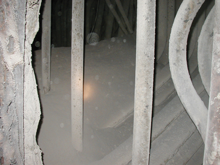
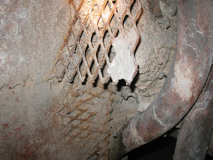
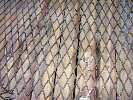
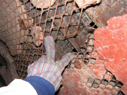
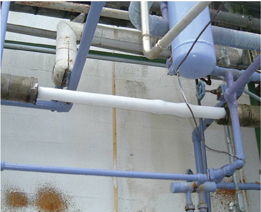
Condition of Existing Insulation Systems

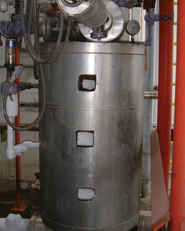
Based on visual inspection, it was estimated that 70 percent of the existing insulation system is in some stage of failure. The newer insulation systems (installed in the last 3 to 5 years) appear to be performing satisfactorily, while the older insulation systems (5 to 25-plus years in age) have failed for multiple reasons.

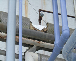
The failed insulation systems are problematic for a number of reasons, including the following:

  • Corrosion of the substrate under the insulation could result in an ammonia release.
  • The increased weight of the wet insulation and/or ice could cause the piping or equipment to exceed the structural design of their support systems.
  • Continual dripping of water from the insulation and/or melting of the ice on the insulation system could create a personnel safety concern.
  • The wet insulation has contributed to the development of mold.
  • The failed insulation systems have resulted in increased energy consumption and greenhouse gas emissions.
  • The reduced efficiency of the insulation system is not allowing the refrigeration and other equipment to function as designed, resulting in decreased plant productivity and/or increased cost of production.
  • The failed insulation systems are increasing annual operating cost and life-cycle costs.

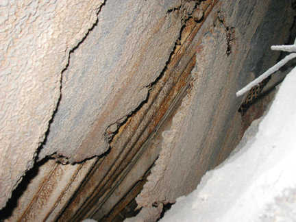
Why Has the Insulation System Failed?

Pinpointing the exact cause by location and approximate time a failure occurred is difficult, especially since even the slightest area of damage can easily lead to more extensive damage over a broader area. The following list does not rank items in order of importance; a combination of these occurrences has led to current conditions.

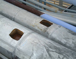
Non-destructive testing: Anytime an insulation system is penetrated, the integrity of the overall system is compromised, especially on services below ambient temperatures. The problem is compounded when the area penetrated is not properly repaired in a timely fashion. All areas tested showed extensive failure of the insulation system.

Weather damage: Damage created by weather (hail and wind) was noted in some areas.

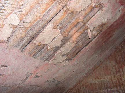
Insulation system design: Old specifications were not available for review. However, areas were noted where the insulation thickness was not adequate, vapor barriers were not installed, an outer jacket was not installed, penetrations were not properly addressed and sealed, and outer jacket lap areas were not correctly located. Was the insulation design the problem, or was it improper application? The answer is probably that both contributed to the problem.

During the inspection process, the use of multiple insulation systems was noted. Given the diverse reasons for and the magnitude of the insulation system failures, it is impossible to point to a given insulation system as the problem.

Lack of maintenance: The importance of maintenance is dramatically increased on insulation systems operating below ambient temperature and exposed to weather. A proper and aggressive insulation system maintenance program would have substantially reduced the extent and severity of the problem at a net lower cost over time.

Economic Analysis

The economic analysis of the insulation systems comprised five tasks:

  1. Identifying the appropriate operating and ambient conditions for the analysis
  2. Estimating the cost to remove unwanted heat gains
  3. Estimating the heat gains through the existing insulation systems
  4. Determining the appropriate levels for insulation upgrades
  5. Estimating the savings attainable by upgrading to recommended levels

For purposes of analysis, the refrigeration system piping and vessels fell into one of the following three categories:

Low Temperature 9 in. Hg Vac. -40°F
Low-Medium Temperature 20 psig 5°F
High-Medium Temperature 35 psig 22°F

In addition, the stainless steel juice lines were assumed to operate at a temperature of 34°F.
While there are certainly variations from these levels based on special cases and normal process variation, these three levels were chosen to describe the operating temperatures found in the system. For outdoor conditions, annual energy calculations on the average annual temperature as reported in the National Climatic Data Center CLIM20 Report were used.

Temperatures in the ventilated engine rooms vary but, on average, are somewhat higher than the outdoor air due to the heat release from equipment. It was estimated an average 5°F differential for an average annual indoor temperature of 77°F with a wind speed of 1 mile per hour (mph).

Freezers are maintained at an average temperature of -5°F or 20°F (depending on the service), and coolers were assumed to be 35°F. Average wind speed of 1 mph was assumed for these indoor applications.

Cost of Removing Unwanted Heat Gains

A key part of an insulation energy appraisal is determining the cost of unwanted heat gains. This involves determining not only the cost of the electricity, but also how efficiently that electrical energy is used. For a refrigeration system, the utilization efficiency is expressed as the coefficient of performance (COP), the benefit of the cycle (amount of heat removed) divided by the required energy input to operate the cycle. The key variables for this complex system were the high-side (condensing) and low-side (evaporating) temperatures of the system.

High-side (condensing) temperatures are determined by the ambient weather conditions and condenser design. The facility uses evaporative condensers. The condensing temperature varies between 80°F and 100°F. For purposes of this analysis, an annual average of 90°F was assumed. (This translates to a condensing pressure of 165 psig.) Low-side (evaporating) temperatures are 40°F (Low Temp), 5°F (Low-Medium Temp), or 22°F (High-Medium Temp).

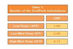
COP estimates were calculated for each of the three suction levels using a public domain refrigeration analysis package (CoolPack). For purposes of this calculation, it was assumed that the low-temperature loads use a two-stage system with flash intercooler, while the medium-temperature loads use single-stage systems. The CoolPack software uses a number of default assumptions (e.g., compressor efficiency, pressure drops in piping, liquid overfeed ratios, degree of subcooling of condensed liquid), so the results should be viewed as estimates based on similar systems. Results of the CoolPack calculations are in Figure 6.

Note that the estimate of the COP for the low-temperature system is roughly half the COP of the medium-temperature systems. Also, note that the temperature difference (ambient-operating) for the low-temperature systems will be roughly twice that of the medium-temperature systems. Therefore, the economic value of insulation on the low-temperature piping and vessels should be roughly four times that for the medium-temperature systems.

The facility purchases most of its electrical power from a local utility company and takes advantage of the time-of-day rates by shutting down some of the refrigeration equipment during peak periods and restarting during off-peak periods. For confidentiality reasons, the actual energy cost is not discussed in this article, but it is safe to assume the net cost is considerably lower than market rates. Thus, all savings estimated in the assessment would be substantially higher if market rates were applied.

Estimating Heat Gains

Estimating heat gains through the existing insulation system cannot be done with precision. It is possible, however, to make educated guesses about the condition of the existing insulation system and to estimate the overall performance of the system. These estimates can then be compared to estimates of the performance of upgraded systems.

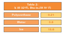
It is estimated that 70 percent of the existing system at the facility is in some stage of failure. Specifications and literature on the older insulation systems were not available, so it was assumed that the 30-percent undamaged portion of the system is performing at a level of 90 percent of the thermal resistance of commercially available polyisocyanurate insulation. (Note: Other insulation systems could also have been used for these calculations.) To estimate the performance of the 70-percent failed portions of the system, it is helpful to compare the thermal conductivity of the “de-rated” polyurethane insulation to liquid water and to ice.

If the existing insulation were completely saturated with water, the heat gain would be roughly 18 times (3.8 ÷ 0.21) the heat gain for a dry system. If it were completely saturated with ice, the heat gain would be roughly 74 times (15.6 ÷ 0.21) the heat gain for a dry system.

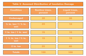
Considering that the operating temperatures of the piping and vessels are below freezing (with the exception of the juice lines), it is reasonable to assume that some portion of the liquid water will have frozen. Certainly, any missing or uninsulated portions will quickly become ice covered. Based on this reasoning, “weighted average” heat gains were developed based on the assumptions in Figure 8.

Juice lines are assumed to be 30 percent undamaged, 35 percent half wet, and 35 percent completely wet.

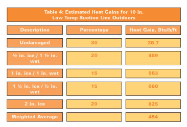
These assumptions were used, along with the 3E Plus® computer program developed by the North American Insulation Manufacturers Association (NAIMA), available at www.pipeinsulation.org, to develop estimates for heat gains for each of the operating temperatures, sizes, and locations throughout the facility. To illustrate, consider a 10-inch NPS (nominal pipe size) low-temperature suction line running outdoors (see Figure 9).

Based on this set of assumptions, it was estimated that a typical existing 10-inch NPS suction line outdoors will have, on average, a heat gain of 454 Btu/h/ft. This process was repeated for each of the line sizes, operating temperatures, and locations identified in the facility.

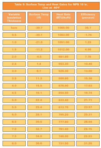
Note that the estimate assumes a 2-inch thickness of existing insulation with a weathered aluminum jacket throughout the site. Some lines, however, were uninsulated or had significant portions of insulation missing and significant buildup of ice. A logical question is whether the 2 inches of ice assumption is valid for the uninsulated portions of the lines. The 3E Plus software was used to explore this question by customizing the program to include ice as an insulating material. Results for a 10-inch NPS low-temperature (-40°F) outdoor suction line are summarized in Figure 10.

Focusing on the Surface Temperature column, note that at a thickness of 2 inches of ice, the predicted surface temperature is -4.5°F. In central Florida, the dew-point temperature rarely drops below 20°F. So at a thickness of 2 inches of ice, condensation on the outer surface would be expected, and this condensed water would also be expected to freeze, causing the ice layer to grow. Again referring to the Surface Temperature column, note that the surface temperature does not get above the freezing point of water until a thickness of 7 inches is reached. However, the 3E Plus calculation does not account for a number of factors in this situation, namely solar incidence, the latent heat of the condensing water, and the effects of gravity. In addition, outdoor temperatures and wind speeds will not be constant, so some melting will occur, limiting ice buildup to thicknesses less than the 7 inches suggested by the 3E Plus calculations.

Referring to the heat gain column in Figure 10, note that for a 7-inch-thick layer of ice, 3E Plus calculates a heat gain of 761 Btu/h/ft. For a 5-inch thickness, the heat gain is 833 Btu/h/ft. Referring to Figure 6, the estimated heat gain for 2 inches of insulation saturated with ice was 825 Btu/h/ft. Thus, it seems reasonable to use the 825 Btu/h/ft value to represent the heat gain for either the 2 inches frozen case or the uninsulated, ice-covered condition. This result is due to the fact that the heat gains are not very sensitive to the thickness of ice present—ice is a very poor insulator.

To explore this point further, compare the heat gain in Figure 10 for a ½-inch thickness of ice to that for a bare surface. The presence of ice on the surface is predicted to increase the heat gain to the pipe. The estimated heat gain for a bare pipe is 1,065 Btu/h/ft, while the heat gain for a pipe with ½ inch of ice buildup on the surface is 1,083 Btu/h/ft. This is an increase of 1.7 percent over the bare case, because the thin layer of ice adds very little thermal resistance to the system, yet the presence of the ice increases the radiant heat transfer to the outer surface. Ice has a very high emittance (0.97), so radiant heat transfer at the surface is increased over that for bare steel (0.8). The net result is an increase in heat gains for thin layers of ice.

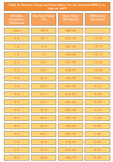
It is interesting to repeat the calculation for the smaller liquid line sizes. Consider the results shown in Figure 11 for a 2-inch NPS low-temperature liquid (-40°F) line exposed to outdoor conditions.

In this case, the heat gain increases from the bare case to a maximum at a thickness of about 1.5 inches and then decreases slowly with additional ice buildup. Note that a thickness over 4 inches would not be expected since the surface temperature would be above the melting point of ice. At 4 inches, the heat gain is roughly 7 percent higher than for a bare pipe.

This interesting result is due not only to the increase in the surface emittance of the ice-covered surface, but also due to a phenomenon known as the critical radius. Although the resistance to conduction increases with the additional thickness of ice, the surface resistance decreases due to increased outer surface area. The maximum heat flow occurs at a thickness corresponding to a critical radius. Further increases in thickness of the ice layer reduce the heat gain.

The bottom line relative to the insulation appraisal is that ice adds little resistance to heat transfer and, in some cases, may actually increase the heat gain to the refrigeration system.

Determining Appropriate Levels for Insulation Upgrades

Insulation on refrigerant piping serves multiple design objectives, including the following:

  • Process control
  • Condensation control
  • Energy conservation (cost and greenhouse gas emissions savings)

For refrigerant piping systems, condensation control usually dictates the appropriate insulation thickness. Process control in refrigeration systems is important, particularly for liquid feed lines where excessive heat gains can result in flash gas and possible pump cavitation.

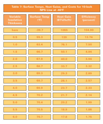
The low-temperature piping system will have both the highest heat gains (due to the high temperature differences between ambient and operating temperature) and the lowest COP. This “high-value” system was therefore selected for initial economic analysis. Results of 3E Plus calculations on low-temperature 10-inch NPS outdoor piping insulated with polystyrene insulation (other types of insulation could have been used for this calculation) with an aluminum jacket are summarized in Figure 12.

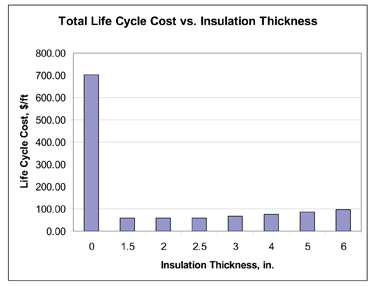
The results associated with the “bare” case should be disregarded. As discussed earlier, a bare steel surface at a temperature of nearly -40°F in central Florida would quickly be covered with several inches of ice, so this case is not very meaningful. The point is that a relatively small amount of insulation (½ inch) reduces the heat gain significantly and raises the surface temperature to about 55°F. The cost of removing that heat gain drops to $13.74/ft/yr. Adding thickness reduces heat gains and associated operating costs further, but at a decreasing rate. The problem becomes one of determining the optimum thickness from a life-cycle cost (LCC) basis. This optimum thickness (sometimes called the economic thickness) is the thickness that minimizes the total costs (initial installed cost plus operating costs) over the life of the insulation system.

Determining the economic thickness is not easy since it depends on a number of factors that are unknown or unknowable. However, it is possible to make estimates based on a set of assumptions. An example calculation is summarized in Figure 14. For the purposes of this analysis, an economic life of 10 years and an annual discount rate (cost of money) of 8 percent was assumed. This set of economic assumptions translates into a multiplier (the Uniform Present Worth Factor, or UPWF) of 6.71 on the annual operating costs.

For the purposes of this analysis, installed costs were estimated using the FEA Method built into the 3E Plus program. Material cost factors of $6/ft for 2 x 2 pipe insulation and $2/ft2 for 2-inch board insulation were used, along with a labor rate of $60/hr. These cost estimates do not include an allowance for removal and disposal of existing insulation or the inspection, repair, and preparation of the substrate. Also note that these costs may vary based on a number of factors.

In this case, a thickness of 2 inches of insulation yields the lowest life-cycle cost of $58.77/ft/yr, so this is the economic thickness. Note that the estimated operating costs at a 2-inch thickness are $3.94/ft/yr. Increasing the thickness to 2 ½ inches is estimated to save an additional $0.62/ft/yr, or $4.16/ft over the life cycle. The installed cost of the additional ½ inch is estimated at $4.49/ft, so the additional ½-inch increment is not economically justified. However, the optimum is broad. Life-cycle costs do not vary more than 10 percent from 1 ½ to 3 inches. Also, simple payback (relative to the bare case) is less than a year for all the cases examined.

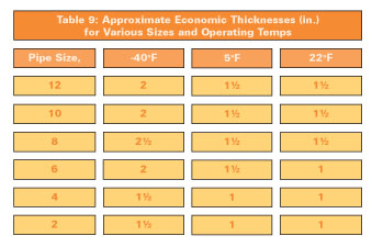
The process was repeated for other sizes and operating temperatures; results are shown in Figure 15.

The conclusion is that the economic thicknesses are lower than the condensation control thicknesses and, accordingly, condensation control will determine the appropriate levels for upgrades.

Selecting the insulation thickness based on condensation control does not mean that the system is somehow “uneconomic.” It simply means that the economic return is less than the maximum possible. Referring to Figure 14, note that the condensation control thickness is 6 inches, while the economic thickness is 2 inches. At 6 inches, the simple payback is 0.8 years (10 months) relative to the uninsulated case. At this thickness, the present value of the savings over the life of the investment is $692/ft. This compares to an initial installed cost of $87, so the net present value is $605/foot. This does not include the economic value of controlling condensation. If a dollar value could be assigned to this benefit, the net present value would be higher.

Estimating Savings From Upgrades

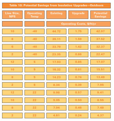
The final step in the assessment consists of calculating the expected performance of upgrades to the insulation system. As discussed above, the calculations assume upgrades to the thicknesses and materials recommended by the facility. The thermal conductivity curve appropriate for this insulation material was utilized in the 3E Plus program. Results on a per-foot basis for outdoor piping are summarized in Figure 16.

As expected, the greatest potential savings are for the low-temperature lines, due to the combined effects of greater temperature differences and the lower COP for these systems. Savings estimates for vessels range from $1.57/ft2/yr for the 22°F vessels to $8.50/ft2/yr for the low-temperature (-40°F) vessels outdoors.

These savings estimates depend strongly on the assumptions made about the performance of the existing insulation system. Recall that the existing performance was based on the “weighted average” of a mix of conditions. Savings for upgrading uninsulated lines will be greater than these values.

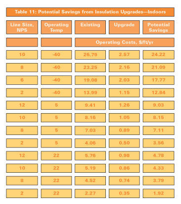
Estimates for the indoor lines are summarized in Figure 17. Savings from upgrading indoor lines are generally lower due to the lower heat gains expected for existing indoor lines and the lower insulation thicknesses assumed for upgrades.

Insulating lines and vessels inside coolers and freezers will not generally translate into energy savings since these heat gains are beneficial (removal of thermal energy from the cooler or freezer). However, insulation in these locations is important from a process control, safety, and housekeeping standpoint.

Based on rough estimates of the quantities of piping and vessels judged to need upgrading (approximately 10,000 linear feet), it was estimated that the potential aggregate annual savings are $110,000. The associated reduction of CO2 emissions is estimated to be about 1,010 metric tons per year.

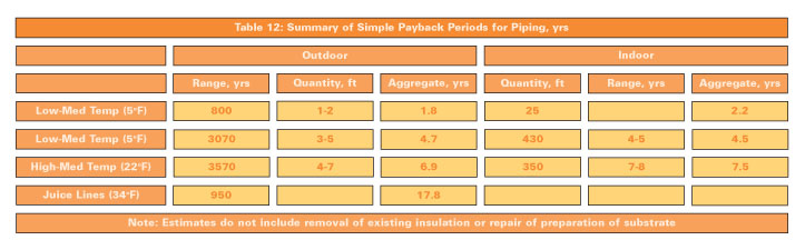
The simple payback periods associated with upgrades will vary depending on the cost and the scope of the upgrades. Upgrading damaged or missing sections of low-temperature lines and vessels outdoors will pay back in 1 to 2 years. Payback periods for the medium-temperature surfaces will be longer. Payback periods for specific surfaces are summarized for piping in Figure 18.

The higher temperature surfaces have longer payback periods due to the combined effects of smaller temperature differences between the ambient and operating fluids, and the higher coefficient of performance associated with these lines. Also, these payback periods take into account the thermal benefit of the existing insulation system, including wet and frozen insulation. Payback periods for uninsulated lines or lines with missing insulation will be shorter.

The Bottom Line

Properly designing, installing, and maintaining any mechanical insulation system—especially systems operating below ambient conditions—can provide a significant return on investment beyond that of a simple payback calculation. Management at this citrus facility chose to examine its existing insulation systems, and the assessment results yielded a roadmap for continuous improvement.

The authors offer congratulations to the management at this facility on their foresight and extend our appreciation to them for allowing us to share their story. Does your facility have a similar story? If so, please e-mail editor@insulation.org.
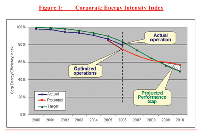
Figure 1

Insulation is missing on this liquid line.

Figure 2

The insulation and vapor retarder are both damaged.

Figure 3

These rooftop lines have unrepaired access in a “catch rain” position.

Figure 4

There are multiple inspection locations on this cold vessel.

Figure 5

This jacket and vapor retarder were damaged by weather.

Figure 6
Figure 7
Figure 8
Figure 9
Figure 10
Figure 11
Figure 12
Figure 13
Figure 14
Figure 15
Figure 16
Figure 17
Figure 18

Increasing population density and mobility, and mechanization of workplaces, households, and leisure activities, have resulted in increased general noise exposure for most people. The consequences for many are concentration and sleep disturbances, noise-induced hearing loss (noise deafness), and damage to the nervous system in the form of stomach, heart, and circulatory problems. According to statistics from the European Agency for Safety and Health at Work, approximately 22.5 million people in Europe suffered from hearing impairment due to noise in 2001, and about 2 million were considered extremely deaf. The costs of hearing impairment have been estimated at EUR 78 billion per year. Noise deafness is regarded as the most important and most recognized occupational disease, predominantly affecting men who work in manufacturing, construction, and transportation.

The general increase in exposure to noise has raised interest in the issue of noise protection and acoustic problems. The Acoustic Commission of the European Federation of Associations of Insulation Companies (Fédération Européenne des Syndicats d’Entreprises d’Isolation—known as FESI) deals with these problems and assists its members with regard to acoustics and noise protection by providing information, including a series of six documents that address noise and noise protection. The documents can be used as a reference by planners, craftsmen, and contractors, but they are also applicable for training and studies. They provide detailed information about materials and systems and help users understand, evaluate, and solve acoustic problems. The idea behind the documents is to form a bridge between international directives and standards and practice-oriented application.

Document A2: Basics of Acoustics

Acoustics is the science of sound and its influence on human beings. Document A2 deals with physical and physiological basics such as origination, propagation, and sensation of noise. The simple calculation with sound levels, representation of noise weighting, and evaluation criteria forms the basis of acoustic planning and implementation of effective noise protection (see Figure 1). The range of audibility to the human ear and the sensation and effect of different noise situations are shown in Figure 2.

Sound propagation in air, solids, and liquids—i.e., airborne, structure-borne, and water-borne sound—as well as description values for frequency, sound velocity, and wave length for sound events in these media are described in detail. Tables provide necessary material data and numerical values.

Noise characteristics such as complex total sound, tone, and bang are comprehensively explained, as they are the basis of the physiological time, frequency, and nuisance weighting of noise. Explanations are provided for the following noise description values:

  • Sound pressure and sound pressure level
  • Sound velocity and sound velocity level
  • Sound intensity and sound intensity level
  • Sound power and sound power level

The connections between these values also are explained, as is the level arithmetic—i.e., adding, subtracting, and the space and time averaging of sound levels.

Document A3: Product Characteristics—Acoustic Insulation, Absorption, Attenuation

Materials, their characteristics, and their acoustic effects are the subjects of Document A3.
Acoustic insulation, attenuation (absorption) properties of materials, systems, and special constructions are presented and discussed. The international character of the FESI Acoustic Commission guarantees that products, systems, and materials common in Europe are considered.

Sound insulation and sound attenuation of airborne and structure-borne sound, their measurement in the laboratory, and the handling of the single values Rw and R’w are comprehensively explained using figures and examples. Simple calculations for single systems (plane walls or pipes) enable rough estimation of the acoustic insulation of corresponding monolithic systems like brickwork, concrete walls and ceilings, or sheet-metal constructions. Weaknesses of material and system are taken into consideration. Information about “double systems” (basic walls with insulation) and absorbent insulations (suspended ceilings) is important for contractors in the room and building acoustics industry.

The effects of materials and dimensions, resonances, and coupling of single layers with each other are described. Calculations and theoretical considerations are completed and supported by numerous measured values taken from standards, laboratory tests, and literature, providing a summary.

Document A4: Acoustics in Buildings

Document A4 describes sound transmission in buildings, noise protection between rooms and against outdoor noise, as well as problems of ventilation and other operating noises. Consulting engineers and contractors get useful hints for the correct execution of noise-protection measures to avoid possible sources of defect and to determine the effectiveness of noise-control measures.

One precondition for the design and dimensioning of noise protection with regard to building acoustics is knowledge of sound transmission paths (airborne, structure-borne, and impact sound). Document A4 gives examples for sound transmission between rooms through the building structure, as well as along and through technical devices (air conditioning). Simple calculation formulae and given loss factors are provided to enable users to estimate insulation and sound-improvement indices.

Diagrams provide information about the influence of leak points such as venting slots and keyholes on the acoustic insulation of walls, doors, and enclosures. Examples of systems and comprehensive tables with insulation coefficients of approved constructions also are included. Tables with detailed information and classifications of door and window constructions relating to sound insulation provide useful tips.

Document A5: Acoustics in Rooms

Apart from protection against noise, acoustics also involves communication and information so that people in a room can hear and understand what is being said. Document A5 describes acoustic characteristics of rooms and how to influence these characteristics.

The document also explains the physical quantity “reverberation time T” as well as “indices for the determination of speech intelligibility:”

  • Articulation index (AI)
  • Sound interference level (SIL)
  • Percentage articulation loss of consonants (%ALCons)
  • Speech transmission index or rapid speech transmission index (STI, RASTI)

The validity of these quantities, correlations, and proportions, as well as numerous requirements and recommendations, facilitate the weighting of speech intelligibility in different rooms. Subjective factors such as distinctness, spaciousness, harmony, and steadiness also are discussed.

Especially helpful is the table “Key parameters suggested for different types of rooms,” which states by which quantities different types of rooms must be weighted. Subsequent chapters of the document provide details for the treatment and furnishing of rooms.

Simple calculations of sound propagation in rooms of different dimensions (cubic, flat, or long) are provided, along with comments regarding natural frequencies, sound diffusion, and acoustic phenomena like echoes/flutter echoes. Noise protection measures and their materials and position in the room are described so the best possible effect will be achieved.

Document A6: Industrial Acoustics

As EU rules with regard to noise at the workplace and industrial plants’ effects on surrounding neighborhoods have become stricter, Document A6 is of particular importance. Contractors get significant information on the sound and vibration effects of machines and plant components, sound propagation in workshops or toward adjacent residents, and the execution of effective sound protection. Materials, systems, their dimensioning and effect, sources of defects, and problematic situations are also discussed.

Document A6 first deals with sound propagation in free field; in rooms; and in ducts, pipes, and air-conditioning systems. It explains how the distance between sound source and receiver, distribution of the radiated sound energy, acoustic insulation and attenuation on the propagation path, and additional noise sources disturb the “receiver”—e.g., at the workplace or in the neighborhood of a plant. Simple calculations, tables with sound insulation and attenuation, and data of noise sources—e.g., in pipes and air-conditioning systems—enable estimation of disturbing noise and its reduction.

A chapter on noise control discusses measures at the source or the point of origin, at the propagation path, and at the receiver corresponding to the model source, path, and receiver. Measures at the source and on the propagation path have first priority. The chapter describes the function and construction of silencers, sound hoods, and sound screens. Their effect can be estimated by a simple function, or it can be taken from corresponding tables.

The effect of a sound hood is determined by:

  • Structure and weight per unit area of the hood wall
  • Portion of free openings in case of penetrations, or openings for material supply and removal, and
  • Possible vibration transmission by the foundation

Table 9, “Orienting construction characteristics for the enclosure groups,” lists examples and minimum requirements to comply with desired insertion losses. Users get the desired information at a glance without time-consuming calculations.

Absorbent wall or ceiling linings prevent or reduce sound reflections without influencing the direct sound. The effect of this noise protection measure depends not only on the material and its dimensions, but also on the position with regard to noise source and receiver. A figure is provided illustrating such a situation (see Figure 3). The effect of the measure can be estimated with the corresponding functions.

Document A7: Guidance through FESI Documents A2 through A6

Document A7, currently in progress, will be a reference for users of the other documents and includes all terms, rules, and body of directives. The chapter “Noise Control” references significant chapters of aforementioned acoustic documents, standards, and recommendations for further reading on dimension noise protection measures. The chapter “Measurements” describes how to prove the effectiveness of such measures, appropriate procedures and the use of the body of directives (regulations, standards, and recommendations) to determine sound emissions, as well as frequency-dependent weighting and evaluation. In short, document A7 will provide a framework for acoustical design and problem solving.

Future Projects

Apart from completion of Document A7, the Acoustic Commission is dealing with the subject of acoustic comfort. The preparation of Document A5 with the acoustic evaluation of rooms according to their use (e.g., restaurants, classrooms, multi-purpose rooms) and terms like speech intelligibility and distinctness revealed that this subject has not been sufficiently considered in Europe.

Thus, the Acoustic Commission first will verify the situation in Europe through use of a survey in the member countries, which will be supplemented by data of research and science, if necessary. Based on the results, recommendations will be given to standard organizations, working groups, and FESI members to enable them to design and implement noise-protection measures.

Documents A2 through A6 in English and the bilingual edition (German/English) can be downloaded from the FESI website.

Figure 1
Figure 2
Figure 3
Figure 4

Energy efficiency first entered the public consciousness in the mid-1970s in the aftermath of the first “oil shock,” as the consequent high inflation eroded the purchasing power of the average family in oil-importing nations. Once some measure of price stability was restored, however, and the economies adjusted to higher oil prices, energy concerns receded into the background.

After nearly 3 decades, energy supply security and costs recently returned to the limelight, with international oil and gas prices more than doubling over the past year. As high prices have begun to adversely affect corporate bottom lines—especially for energy-intensive industries such as oil and gas, chemicals, and pulp/paper—energy conservation is once again attracting management attention. Unfortunately, there is no quick fix for this situation. Successful energy conservation (or, more appropriately, energy optimization) is a long-term effort: a marathon, not a sprint. Success requires sustained commitment.

On the positive side, there has been tremendous innovation in both the efficient conversion and use of energy. Many new products, design techniques, and operating practices have been developed in both academia and industry that offer the potential to significantly slash the energy intensity of virtually all manufacturing processes, reducing their carbon footprint (i.e., greenhouse gas emissions).

An established body of literature documents the methods and benefits of what could be called “conventional” technical approaches that address the more obvious areas for improvement.

  • Insulation of equipment and piping
  • Steam-trap management—proper selection, monitoring, and maintenance
  • Compressed air management—leak detection and repair, pressure optimization
  • Boiler/furnace efficiency improvement via excess air control, burner modifications, leakage reduction, etc.
  • Multiple effect evaporation—well known in pulp/paper but less in other industries
  • Heat pumps (thermal and mechanical)
  • Preventive maintenance of rotating machinery (pumps, compressors, steam turbines) based on condition and efficiency monitoring
  • Motor replacement—right-sizing, high-efficiency motors
  • Heating, ventilating, and air-conditioning (HVAC) upgrades—better controls
  • High-efficiency lights and lighting management
  • Power factor correction
  • New types of equipment design—e.g., dryers, low-P filters, etc.

The vast majority of industrial energy programs started over the past 25 years have focused on the foregoing tools and techniques. While these are undoubtedly positive steps, in most cases the cumulative savings potential is limited to a relatively meager 5 to 10 percent of the base-case energy intensity.

To capture truly significant savings—on the order of 15 to 50 percent—advanced optimization techniques developed over the past 20 years encompassing both design and operational best practices must be employed.

  1. Operational Optimization
    1. Optimum load management (for series/parallel networks of multiple equipment types—pumps, compressors, turbines, boilers, furnaces, heat exchangers, etc.)
    2. Monitoring of fouling rates in critical heat exchangers, and optimum cleaning schedules
    3. Floating-discharge-pressure compressor control
    4. Multi-variable controls (MVCs)
    5. Optimal control of combined heat and power (CHP) systems (see item 2d under “Design Optimization”)
    6. Optimum driver selection for rotating machinery (fixed-speed motors, multi-speed motors, motors with variable frequency drives [VFDs], steam turbines, gas turbines)
    7. Monitoring and targeting, including development of equipment energy performance indices (EPIs) and overall process/product/plant energy key performance indicators (KPIs). Data collection and quality is a critical issue.
  2. Design Optimization
    1. Identifying relatively minor process modifications, such as small adjustments in operating pressure or temperature of critical reactions and separations (e.g., distillation, evaporation) that could have a major impact on the energy targets for the process
    2. Optimum design of heat exchanger network (HEN) structures, using Pinch Analysis (described below) combined with math programming (mixed integer linear programming, genetic algorithms, etc.)
    3. Identifying the optimum combination of site utilities (cogeneration type, steam pressure levels, hot oil loops, refrigeration levels and refrigerant selection, etc.) that will result in the lowest operating cost, using Pinch Analysis
    4. Optimum design of the CHP system structure, including cogeneration using simulation models based on the results of item 2c (A key element is introducing new degrees of freedom to support items 1e and 1f under “Operational Optimization.”)
    5. Evaluation of adjustable speed drive applications (whether VFDs for existing motors or replacement with a steam turbine drive)

Probably the most significant development of the past 30 years since the first oil shock has been Pinch Analysis. It burst onto the scene in the late 1970s and captured the imagination of the international chemical engineering community with its elegant synthesis of thermodynamic rigor and graphical techniques to solve the hitherto intractable “structural optimization” problem using simple heuristics. Imperial Chemical Industries (United Kingdom) and Union Carbide Corp. (United States) were the early pioneers. By the mid 1980s, a torrent of literature on new advances and industrial success stories was pouring out from both universities and industry.

Many companies jumped on the new bandwagon, but most of them found success elusive. Gradually, but not surprisingly, Pinch Analysis developed an undeserved reputation for being just another passing fad oversold by unscrupulous consultants seeking a quick buck.

Although it is undeniable that some consultants were indeed underqualified, it is instructive to examine the reasons why some companies achieved spectacular success while others failed miserably. From this author’s 20 years of experience in the energy business, both as a buyer and seller, the evidence is clear that most of the failures can be attributed to critical mistakes on the part of senior management.

  • Believing that because Pinch Analysis was easy to understand at a theoretical level, it would be easy to apply at a practical level. Attending a 1-week course on the subject does not render the student an expert. It takes at least two to three projects’ worth of experience to use the software and apply the methodology correctly.
  • Expecting that identification of energy optimization opportunities would automatically result in project implementation.
  • Underestimating the vital importance of reliable data and a supporting infrastructure.
  • Denying corporate energy teams adequate resources in terms of authority, staffing, budget, and time to do the job properly.

Good technology, while necessary, is not sufficient to ensure success. It must be supported by a comprehensive, organization-wide program that removes institutional barriers related to legal, financial, and bureaucratic hurdles.

Case Study: Major National Oil Company

This company is the largest crude oil producer/exporter in the world, with a maximum sustained production capacity over 10 million barrels per day of crude oil and 8,000 million standard cubic feet per day of natural gas. The company operates approximately 32 large gas–oil separation plants, 5 wholly owned oil refineries processing 1,600 thousand barrels per day of crude, 5 gas processing plants, and 2 condensate fractionation plants.

From a standing start, the company reduced its energy intensity by 25 percent within 6 years. How did the company manage to achieve such spectacular success despite an untrained workforce, low energy costs (75 cents/MMBtu for gas, 30 cents/MMBtu for fuel oil, and 3.2 cents/kwh for purchased power), high capital costs (generally 1.3 to 1.5 times U.S. Gulf Coast costs), and a national culture based on the conviction that the oil supply is infinite?

It all started in 1997, when one of the company’s engineers attended an energy conference in Houston and realized that the company’s policies and practices were based on incorrect assumptions and urgently needed to be revamped in light of a changing business environment. With support from the Vice President (VP) of Engineering Services, he got approval for an internal, company-wide survey of actual fuel and power consumption. (Historically, energy was considered to be so cheap that the company did not bother to include fuel and power as cost items in their accounting system). Even at the low values assigned to energy by the accounting department, the cost proved to be staggering, approaching $1 billion per year. When this information was brought to the attention of senior management, they committed the required internal manpower and about $1 million in expenses to conduct a more detailed study by a team of specialized energy/management consultants (including the author of this article).

The 8-month study (conducted in 1998 to 1999) included verification of energy consumption, an estimate of economically feasible savings potential (based on quick audits of 12 representative facilities, lasting 1 week each), and an assessment of company policies and practices that should be instituted or modified to ensure success. The principal credit belongs to the company’s senior management, who understood, accepted, and supported virtually all of the resulting recommendations.

A corporate energy policy was promulgated in 2000, and an Energy Management Steering Committee (EMSC) was formed in 2001, with plant-manager level representation, to oversee the program. The company decided to develop core in-house expertise to manage the program and supplement short-term peaks in manpower needs through the use of external consultants. A new Energy Systems Unit (ESU) was established at corporate engineering in 2001, with funding approval for 9 to 12 full-time engineers and an administrative assistant to help implement the EMSC’s strategic plan.

The EMSC developed a 10-year goal (publicized company-wide) to reduce corporate energy intensity by 50 percent compared to the year 2000 baseline, and rolling 5-year plans to achieve the target. The results are a testament to the success of the program. It is interesting to note that even if no further projects are approved, the company will have achieved a 40-percent reduction in energy intensity. Once additional projects—identified but not yet approved for funding—are implemented, the original target of 50-percent reduction in energy intensity by 2010 should be met comfortably.

Credit also must go to the EMSC’s well-conceived and executed strategy, which clearly recognized the importance of non-technical factors. Key elements of the strategy are outlined below.

  1. Optimize facility design and operation through deployment of industry-accepted best practices and economically sound leading edge technologies.
    • Energy optimization of existing facilities (retrofit)
    • Energy optimization of new plant designs
  2. Build a supportive organizational infrastructure.
  3. Promote transparency and accountability through development and deployment of energy KPIs and EPIs.
  4. Develop in-house technical expertise supplemented by outsourcing as needed.

Energy optimization of existing facilities (retrofit basis) was an important first step in establishing credibility for the technical approach and demonstrating that the targets set by the EMSC were realistic and achievable. To begin, the ESU was staffed by one energy consultant recruited from the United States (the author) and four company engineers. All studies were conducted by ESU staff principally as a means to gain experience and build in-house technical expertise. As the workload grew, additional engineers were transferred to the ESU from other parts of the company, and a second energy specialist with Pinch Analysis expertise was recruited from the United States. This multi-year effort helped foster close working relationships and build trust between the plant engineers and corporate staff. When the workload began to exceed in-house capacity, some of the detailed energy studies were outsourced to qualified consulting firms from the United States, the United Kingdom, and India.

One of the key requirements for successful outsourcing is that the buyer should be able to specify the proper scope of work, select the consultants correctly, and negotiate a fair price. It took 3 years for the company to develop skills as a sophisticated buyer. The initial trainees learned to understand the data requirements and knew what to expect in terms of quality of work, schedule, and cost. They were able to redirect the consultants’ work if they felt they were on the wrong track and would make contractual work scope changes on the fly. They knew when to allow more time or money and when not to. Unless the buyer is knowledgeable, or engages a trustworthy consultant, there is high risk that outsourcing can turn into a disastrous experience.

A total of 15 retrofit studies were carried out over 7 years by the ESU. More than 100 company engineers, mostly from the plants, were put through 1- to 2-week training courses in energy optimization that included both technical and management issues. Of these, about 20 engineers who showed interest and promise were put through 1- to 2-year internship programs where they were selected to participate in conducting two or three of the retrofit energy optimization studies. They then became the foundation for new energy teams established at their respective plants.

The results achieved from 2001 through 2006 are summarized in Table 1. One can see that more than 50 percent of the project ideas came from the plants themselves, with technical support from corporate engineering only as needed. The corporate studies intentionally focused on advanced techniques to address the less obvious optimization opportunities, leaving the plant energy teams to focus on more easily implementable “conventional” projects.
The actual overall implementation rate (in terms of dollars) was 54 percent. However, the energy KPIs showed unambiguously that there was a huge variation in performance among the 21 business units: some had implementation rates over 90 percent, while others were below 5 percent. Clearly, the problem lay not in the technical solutions, but in the human factor. This issue is being given top priority in the latest strategic plan.

The company conducted an extensive internal survey in 2007 to determine the root causes for poor implementation and the key predictors of success. The two stand-out success criteria were:

  • Having high-level support, at the Plant Manager and Admin Area VP levels, for energy projects; and
  • Empowerment of plant engineers through providing adequate resources to the energy teams in terms of qualified manpower, training, and budgets that would enable them to prepare credible and properly documented capital budget requests to corporate engineering.

Energy Optimization of New Plants. Once the credibility of the technical approach was established through retrofit studies, the ESU turned its attention to new plants being built by the company—new process units at existing sites and greenfield sites—to try building energy efficiency into the design from the start. While the concept makes perfect sense, they ran into hurdles due to established company practices. The company never did (and still does not) develop its own process designs, but relies on engineering, procurement, and construction (EPC) contractors to provide them. Design/build responsibility lies entirely with the project management organization, where the path to promotion has historically been through only two performance criteria: beat the schedule, and complete under budget. No effort was made to optimize energy costs, which were assumed to be inconsequential. It is no wonder the entire organizational culture became strongly biased toward tried-and-true technologies (i.e., outdated), cutting out any features (e.g., energy efficiency) that could help reduce capital costs. There have even been instances where the contractors simply re-used previous designs from other projects in other countries, without even bothering to change the title blocks on the drawings!

Naturally, all attempts by the ESU to introduce modern, energy-efficient practices met with determined resistance, being rightly seen as having the potential to extend the design schedule and increase capital costs. It took 3 years of personal lobbying with key influential people just to gain initial acceptance of the idea that the correct way to optimize a design was on the basis of life-cycle costs, not first cost. Real-life examples were provided: case studies where energy optimization led to shortened schedules as well as lower capital costs. Once this was accomplished, it opened the door to the concept of optimizing process/utility designs for site-specific conditions and including energy costs as one of the factors that should be included. Ultimately, the requirement for an integrated process-CHP energy optimization study during the front-end engineering design stage was accepted as an internationally accepted, value-improving practice and written into the company standards.

Figure 1

Summary of Identified Opportunities

The development of effective and efficient mechanical insulation systems aboard ships present many challenges to the designer. Ship construction regulations and material certifications are rigid, and strict adherence to performance specifications mandate the insulation system design be validated through rigorous analysis. Additionally, due to the expansion of international trade and U.S. national defense priorities, ocean-going vessels often sail through extreme conditions. The mechanical insulation system designer must be conscious of the limits for both temperature and relative humidity. A single ship may experience limits ranging from summer conditions with temperatures as high as 130°F and 90 percent relative humidity to winter conditions with temperatures as low as 0°F. These regulatory and environmental variables present a formidable challenge to insulation specification seeking to maintain design compartment temperatures throughout the vessel.

Beginning in 2002, one insulation contractor’s new construction project team was tasked to assist in the design of a new shipbuilding program with the ship builder, General Dynamics (GD) NASSCO. This program, named the T-AKE Dry Cargo/ Ammunition Ship, was developed to provide a ship capable of delivering ammunition, provisions, stores, spare parts, potable water, and petroleum products to carrier battle groups and other naval forces, serving as a shuttle or station ship. Achieving the stated mission required several cargo holds that were at times refrigerated to -9°F, as well as other cargo holds maintained at 84°F. Coupled with the extreme design challenge presented by environmental conditions, the contractor and GD NASSCO’s assignment was to design the insulation for the mechanical ventilation systems that would maintain conditioned air temperatures in various compartments and prevent condensation formation on the duct and pipe surfaces.

In 2003 and 2004, the detailed insulation design of the T-AKE program began to take shape. New requirements surfaced regarding insulation thickness of secondary coolant (brine) piping; specifically, American Bureau of Shipping (ABS) Rule 6-2-6/ 23.3.4, which states:

“Secondary coolant piping, valves, and fittings whose working temperature is below the normal ambient temperature are to be effectively insulated. The insulation is to be sufficiently thick to prevent the formation of moisture on the pipe surface at a relative humidity of 90 percent.”

Contractual requirements dictated that GD NASSCO and the insulation contractor provide insulation thickness calculations for the secondary coolant (brine) piping that ensured adequate thickness to prevent moisture formation. Additionally, significant quantities of ventilation ducting traversing multiple compartments now were required to be insulated due to increased air volume movement and rate of changes per hour.

The engineering challenge was to provide acceptable calculations (as contractually required) for the brine piping and condensation prevention/heat loss calculations for ventilation duct. Many calculations were required because the piping and ventilation ducts traversed many compartments, each having specific winter and summer design temperatures, relative humidities, and relative wind speeds, along with variation in pipe and duct size. With the unprecedented volume of calculations required, and the absence of any definitive source to supply the detailed thickness requirements that met the team’s needs, the heat loss analysis computer program 3E Plus® emerged as the preferred design tool.

In their research of 3E Plus, the team learned that ASHRAE had used the software to assign insulation thickness of varying types in its 1998 Refrigeration Handbook, Chapter 32, “Insulation Systems for Refrigerant Piping,” which lent immediate credibility to the design. The project management team had to reach a certain level of comfort that the software would provide consistently accurate thickness recommendations for the variables the team specified. To achieve this goal, the team validated the accuracy by performing a number of manual calculations on dissimilar circumstances. Every manual calculation was within 97 percent of the 3E Plus calculation.

The insulation design for the refrigerated brine system proved exceptionally challenging. As noted earlier, in the calculation of piping insulation thickness, ABS regulations require no moisture formation on the surface of the insulated piping at a relative humidity of 90 percent. As a result, every compartment the brine piping traversed, from the chiller unit locations to the actual cargo space that holds the diffusing equipment, required a separate calculation. The easy road, from a design perspective, would have been to assign one thickness throughout, accommodating the most onerous compartment temperature. During construction, however, this approach ultimately would have led to increased material and labor costs due to confined working areas and condensed pipe runs. From an accuracy and construction viewpoint, it was determined that the best approach was to perform calculations for each compartment through which the brine piping traveled.

Working in concert with the team’s engineering colleagues at GD NASSCO, the insulation contractor compiled the compartment variables necessary to calculate the correct thickness:

  1. Summer or winter season design temperature
  2. Relative humidity
  3. Wind speed
  4. Pipe diameter

Although the regulatory requirements were a contractual obligation, the team’s use of 3E Plus in calculating design insulation thickness also provided a more practical solution: supporting system operation by preventing moisture condensation and intrusion. Based on the design temperatures of the brine system and the compartments through which the system traveled, high vapor pressure was a major concern. The design pipe insulation thickness was fundamental in preventing moisture condensation, accumulation, intrusion to the underlying piping system, and potential insulation system failure. Since the costs to replace the insulation system components in the event of a failure would have been prohibitive, it was critical to do the job correctly. 3E Plus provided the team with the detailed calculations necessary to ensure regulatory approval and the confidence that the prescribed thickness would perform as required under the extreme shipboard conditions.

Heating, ventilation, and air-conditioning (HVAC) functions for shipboard applications are similar to land-based treatments, as they control temperature, humidity, and quality of the air in the various spaces on the vessel. Shipboard HVAC system types also vary based on the ship class. In this scenario, the T-AKE vessels use terminal reheat systems. One unique design consideration is that ships operate in a wide range of weather conditions and can be subjected to large variations in climates within short periods. There are also various climates inside these ships. For example, on T-AKE vessels, there are more than 750 compartments with varying HVAC requirements, utilizing more than 50 air handlers with off-coil temperatures designed to meet their specific needs. These compartments vary in use from machinery spaces to air-conditioned cargo holds and accommodations, including living or service spaces.

The insulation design prevents condensation and limits sensible heat added to or extracted from the air in the duct as it passes through the various compartments on its path to the final destination. The most stringent design calculations were based on the specification requirement to install insulation on parts of air-conditioning systems where the space dew point is more than 4°F higher than the duct air dry bulb temperature. There also were requirements for treatment on any outside air passing through air-conditioned spaces and supply systems inside machinery rooms. The team had to define the required treatments on each duct run based on the scenarios that existed. By using 3E Plus to perform these calculations, the team ensured that the systems were not under-insulated, saving material costs in some large areas. Many scenarios were repeated, but without using 3E Plus as the design tool, significantly more time would have been required to determine the proper treatments.

Performance of Insulation Design

The first five vessels of this program have been delivered, with the first three seeing significant tours in support of the U.S. naval fleet. The insulation contractor has been a part of the visual inspection team of one of the delivered ships, and it appears that all insulation systems—particularly the refrigerated brine system and all ventilation ducts—are performing as designed. To date, there have been no reported issues regarding the performance of insulation systems for the brine system or ventilation ducts.

Generally, there has been no negative feedback from the fleet, which suggests that the mechanical insulation systems are working as intended. This further validates 3E Plus as an integral and accurate part of the design efforts.

Conclusion

Insulation design for land-based HVAC systems is, under normal circumstances, a challenge. On ocean-going vessels such as the T-AKE vessels, which travel through a wide variety of climactic conditions, it is an even greater challenge.

The 3E Plus program enabled the mechanical insulation system designers to achieve the optimal insulation design on two key systems for the T-AKE vessel program. This, in turn, allowed the insulation contractor to install reliable and well-designed mechanical insulation systems, thereby maintaining the ship’s intended capabilities and missions.

3E Plus is available free from the North American Insulation Manufacturers Association.

Figure 1

The T-AKE Dry Cargo/Ammunition Ship is designed to deliver ammunition, provisions, and other supplies to carrier battle groups.

Figure 2

A ventilation supply duct and protective screen. The insulation thickness was designed to accommodate the variables for this compartment to prevent condensation formation.

Figure 3

A refrigerated secondary coolant (brine) system manifold. Insulation thickness was designed to allow for adequate pipe clearances while preventing moisture formation.

The Hammerfest Liquefied Natural Gas (LNG) Plant is the world’s northernmost LNG plant, in remote northern Norway, 300 miles north of the Arctic Circle. According to some sources, the Arctic region probably holds 25 percent of the planet’s undiscovered hydrocarbon reserves.

The plant owner, StatoilHydro, commissioned the project. The contractor, a joint venture between Aker Kvaerner and KAEFER Group, carried out the hook-up and installation work in one of the world’s most challenging oil and gas development projects. The installation work on site took 3 years, involving 3,000 workers putting in 5.4 million hours to get the plant ready for operation.

Hammerfest was a “green” project, with all CO2 pumped back to the gas field of SnØhvit. Norway is a reliable energy provider, and StatoilHydro has entered into contracts with American companies for a 20-year period. LNG will be shipped from the Arctic plant in Hammerfest to an LNG terminal at Cove Point, Maryland, on the U.S. East Coast.

The Challenges

Many companies bid on the on-site installation for the Hammerfest plant, which was scheduled to take about 2 years but actually took 3 years. The final cost was $600 million for insulation, passive fireproofing, surface protection, and weather protection.

There were many challenges to overcome. First, the area where the plant was to be built is exposed to extreme weather. Second, there was a total lack of infrastructure and logistics. This was uncharted territory: the first time an entire LNG plant had to be built in modules and large units and then transported by sea to the plant site, several thousand miles from the production workshops.

The key to success lay in creating a controlled working environment. Our part of the job was to insulate the entire plant, for applications ranging from high-temperature to cryogenic. We began by enclosing all the workplaces, concentrating on factors that were important to the working environment, such as the structure and a focus on safety.

The entire plant was constructed in various locations all over Europe and then transported by sea to Hammerfest. Nobody had seen a jigsaw puzzle like this before, because no offshore gas field has ever been developed this far north. The LNG plant in Hammerfest is certainly the world’s northernmost and probably the one most exposed to extreme weather.

The LNG plant was prefabricated far south in Europe, an entirely appropriate process for a project facing such unusual conditions. New ways of construction had to be developed to accommodate the lack of local building capacity and infrastructure, as well as the local climatic conditions. Throughout the process, the operative question was how to put this puzzle together. For example, the heart of the plant was built in Cadiz, Spain, and had to be transported by sea. With the weather conditions on site, however, there was only a 3-month weather window for sea transport.

Because transporting the modules had to be done within the weather window, the job of piecing everything together was much greater and much more complicated for the Aker Kvaerner/KAEFER Group than is typical. The modules and the process plant arrived in a far less completed state than anticipated when the contract was signed. In addition, because parts of the facility were made at a number of locations throughout Europe, quantity variations and quality deviations existed. Bad weather at sea also caused damage to the modules that was only detected upon arrival at the site.

Putting People First

The biggest challenges came from the site itself: How would personnel be able to work in such extreme weather conditions? How could the site be prepared so that up to 3,000 people could work there? How would employees—and management—get physically and mentally prepared for the job?

To ensure good working conditions, a total area of approximately 3.2 million square feet was enclosed under temporary fabric structures. These houses stood up to the weather for 3 years without a single tear.

Aker Kvaerner/KAEFER Group focused on health and safety. Throughout the construction project, they wanted every single one of their employees to feel safe. Before the work started, they prepared their workers for what lay ahead: 3 weeks of working 10-hour days, followed by 2 weeks off. They chartered their own aircraft to handle personnel rotation to and from the site. Project professionals from KAEFER’s companies throughout Europe flew in and out of central hubs on a scheduled air service throughout the contract period.

Whatever the nature of the project, health and safety must be in focus. Systems must be established to capture undesired events. In 3 years, the Hammerfest LNG project had just three small incidents that resulted in lost working time, but no great danger.

Proactive—and visible—management is another necessity. There is a big difference between being well informed and being told. Top management visited the Hammerfest LNG site at least once a month throughout the construction period. Dialogue with employees, clients, and other involved parties was critical.

Lessons Learned

Once Project SnØhvit had been completed, Aker Kvaerner/KAEFER Group got substantial feedback about what they had achieved and the significance of their work for the future. They also were asked what they learned. The lessons included:

  • When prefabrication is involved, follow-up with all the different workshops involved is critical to ensure even quality and enable proper planning for piecing everything together based on the actual level of completion.
  • Logistics should be improved, and there should be greater focus on weather protection during transportation to the building site.

Everyone involved has good reason to be satisfied. The opportunities were there, and the challenges were obvious, but nothing was insurmountable.
The Hammerfest LNG Plant started exporting to the United States in December 2007. After 1 year of operation, no problems have been reported with the LNG insulation systems.

Figure 1

The Northern Lights in green over the illuminated LNG plant, one cold winter night.

Figure 2

Arctic opportunities and challenges in exploration and production of oil and gas in the Arctic United States, Canada, and Russia.

Figure 3

Overview of the construction site and the world’s northernmost city, Hammerfest.

Figure 4

Typical winter weather at the site. The truck looks like an iceberg.

Figure 5

LNG plant layout and the barge with the process plant built as the top side.

Figure 6

Jigsaw puzzle: main fabrication yards and the sea routes from the prefabricated LNG plant to the construction site.

Figure 7

The process plant arriving in Hammerfest on a heavy lift vessel from southern Spain, a voyage of more than 1,200 miles in rough waters.

Figure 8

Heated weather protection houses built to withstand high wind speed and low temperatures.

Figure 9

Heated weather protection houses provided climate-controlled workplaces for all trades on site during the construction period.

Figure 10

KAEFER’s main deliveries to the world’s northernmost LNG plant.

Figure 11
Figure 12